Power spectra computation in HEALPIX pixellisation

Introduction

This tutorial shows how to compute the power spectra of spin 0 and 2 fields. We will use the HEALPIX pixellisation to pass through the different steps of generation. If you are interested on doing the same thing with CAR pixellisation, you can have a look at this file.

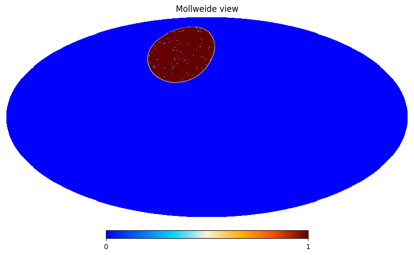
The HEALPIX survey mask will be a disk of radius 25 degree centered on longitude 30 degree and latitude 50 degree, It will have a resolution nside=1024.

We simulate 2 splits with 5 µK.arcmin noise and we also include a point source mask with 100 holes of size 10 arcminutes. We appodize the survey mask with an apodisation of 1 degree and the point source mask with an apodisation of 0.3 degree. We finally compute the spectra between the 2 splits of data up to lmax=1000.

Preamble

Versions used for this tutorial

import healpy as hp
import matplotlib as mpl
import matplotlib.pyplot as plt
import numpy as np
import pixell
import pspy

print("     Numpy :", np.__version__)
print("    Healpy :", hp.__version__)
print("Matplotlib :", mpl.__version__)
print("    pixell :", pixell.__version__)
print("      pspy :", pspy.__version__)

     Numpy : 1.26.3
    Healpy : 1.16.6
Matplotlib : 3.8.2
    pixell : 0.21.1
      pspy : 1.7.0+1.gafa4ce9.dirty

Set Planck colormap as default

pixell.colorize.mpl_setdefault("planck")

Generation of the templates, mask and apodisation type

We start by specifying the HEALPIX parameters for the window function. it will be a disk of radius 25 degree centered on longitude 30 degree and latitude 50 degree, It will have a resolution nside=1024.

lon, lat = 30, 50
radius = 25
nside = 1024

For this example, we will make use of 3 components : Temperature (spin 0) and polarisation Q and U (spin 2)

ncomp = 3

Given the parameters, we can generate the HEALPIX template as follow

from pspy import so_map

template_healpix = so_map.healpix_template(ncomp, nside=nside)

We also define a binary template for the window function: we set pixel inside the disk at 1 and pixel outside at zero

binary_healpix = so_map.healpix_template(ncomp=1, nside=nside)
vec = hp.pixelfunc.ang2vec(lon, lat, lonlat=True)
disc = hp.query_disc(nside, vec, radius=radius * np.pi / 180)
binary_healpix.data[disc] = 1

Generation of spectra

Generation of simulations

We first have to compute a set of theoretical power spectra \(C_\ell\) using a Boltzmann solver such as CAMB and we need to install it since this is a prerequisite of pspy. We can do it within this notebook by executing the following command

%pip install camb

Requirement already satisfied: camb in /home/garrido/Workdir/cmb/development/pspy/pyenv/lib/python3.11/site-packages (1.5.3)
Requirement already satisfied: scipy>=1.0 in /home/garrido/Workdir/cmb/development/pspy/pyenv/lib/python3.11/site-packages (from camb) (1.11.4)
Requirement already satisfied: sympy>=1.0 in /home/garrido/Workdir/cmb/development/pspy/pyenv/lib/python3.11/site-packages (from camb) (1.12)
Requirement already satisfied: packaging in /home/garrido/Workdir/cmb/development/pspy/pyenv/lib/python3.11/site-packages (from camb) (23.2)
Requirement already satisfied: numpy<1.28.0,>=1.21.6 in /home/garrido/Workdir/cmb/development/pspy/pyenv/lib/python3.11/site-packages (from scipy>=1.0->camb) (1.26.3)
Requirement already satisfied: mpmath>=0.19 in /home/garrido/Workdir/cmb/development/pspy/pyenv/lib/python3.11/site-packages (from sympy>=1.0->camb) (1.3.0)
Note: you may need to restart the kernel to use updated packages.

To make sure everything goes well, we can import CAMB and check its version

import camb

print("CAMB version:", camb.__version__)

CAMB version: 1.5.3

Now that CAMB is properly installed, we will produce the \(C_\ell\)s from \(\ell\)_min=2 to \(\ell\)_max=10⁴ for the following set of \(\Lambda\)CDM parameters

ℓmin, ℓmax = 2, 10**4
ℓ = np.arange(ℓmin, ℓmax)
cosmo_params = {
    "H0": 67.5,
    "As": 1e-10 * np.exp(3.044),
    "ombh2": 0.02237,
    "omch2": 0.1200,
    "ns": 0.9649,
    "Alens": 1.0,
    "tau": 0.0544,
}
pars = camb.set_params(**cosmo_params)
pars.set_for_lmax(ℓmax, lens_potential_accuracy=1)
results = camb.get_results(pars)
powers = results.get_cmb_power_spectra(pars, CMB_unit="muK")

We finally have to write the \(C_\ell\)s into a file to feed the so_map.synfast function

import os

output_dir = "/tmp/tutorial_spectra_spin0and2"
os.makedirs(output_dir, exist_ok=True)
cl_file = os.path.join(output_dir, "cl_camb.dat")
np.savetxt(cl_file, np.hstack([ℓ[:, np.newaxis], powers["total"][ℓmin:ℓmax]]))

Given the CAMB file, we generate a CMB realisation

cmb = template_healpix.synfast(cl_file)

Then, we make 2 splits out of it, each with 5 µK.arcmin rms in temperature and 5xsqrt(2) µK.arcmin in polarisation

nsplits = 2
splits = [cmb.copy() for i in range(nsplits)]
for i in range(nsplits):
    noise = so_map.white_noise(cmb, rms_uKarcmin_T=5, rms_uKarcmin_pol=np.sqrt(2) * 5)
    splits[i].data += noise.data

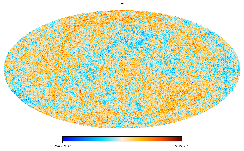
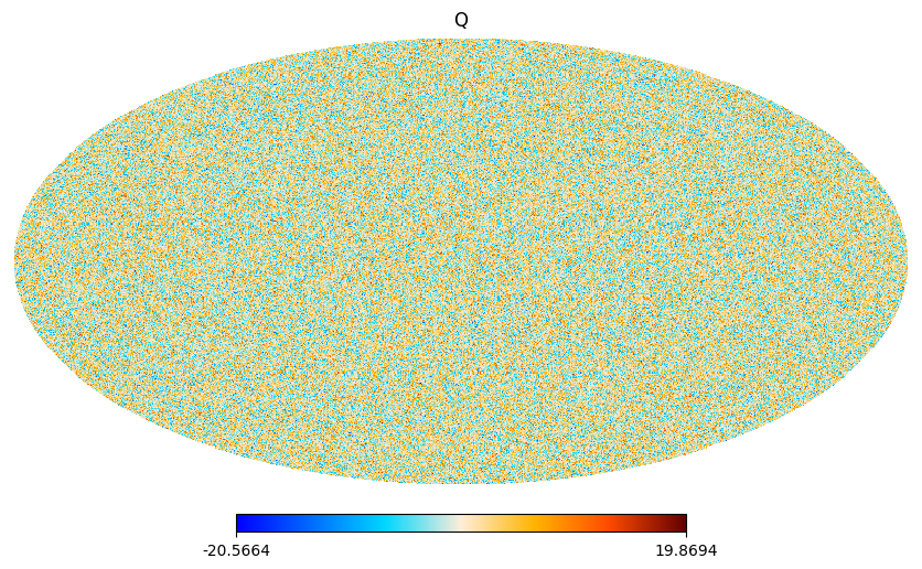
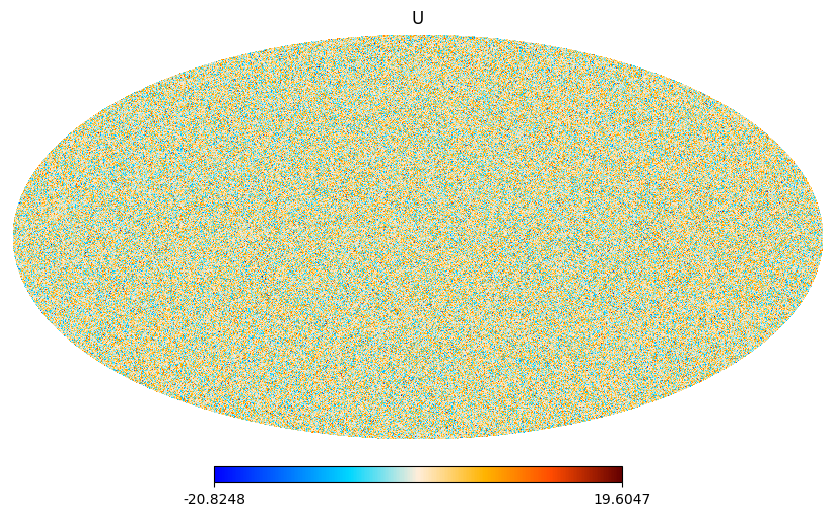
We can plot each component T, Q, U for the original CMB realisation

for i, field in enumerate(fields := "TQU"):
    hp.mollview(cmb.data[i], title=field)

Generate window

We then create an apodisation for the survey mask. We use a C1 apodisation with an apodisation size of 1 degree

from pspy import so_window

window = so_window.create_apodization(binary_healpix, apo_type="C1", apo_radius_degree=1)

We also create a point source mask made of 100 holes each with a 10 arcminutes size

mask = so_map.simulate_source_mask(binary_healpix, n_holes=100, hole_radius_arcmin=10)

and we apodize it

mask = so_window.create_apodization(mask, apo_type="C1", apo_radius_degree=0.3)

The window is given by the product of the survey window and the mask window

window.data *= mask.data
hp.mollview(window.data, min=0, max=1)

Compute mode coupling matrix

For spin 0 and 2 the window need to be a tuple made of two objects: the window used for spin 0 and the one used for spin 2

window = (window, window)

The windows (for spin0 and spin2) are going to couple mode together, we compute a mode coupling matrix in order to undo this effect given a binning file (format: lmin, lmax, lmean) and a \(\ell\)_max value of 1000

from pspy import pspy_utils

binning_file = os.path.join(output_dir, "binning.dat")
pspy_utils.create_binning_file(bin_size=40, n_bins=100, file_name=binning_file)

from pspy import so_mcm

ℓmax = 1000
mbb_inv, Bbl = so_mcm.mcm_and_bbl_spin0and2(window, binning_file, lmax=ℓmax, type="Dl", niter=0)

Compute alms and bin spectra

from pspy import sph_tools

alms = [sph_tools.get_alms(split, window, niter=0, lmax=lmax) for split in splits]

We need to specify the order of the spectra to be used by pspy

spectra = ["TT", "TE", "TB", "ET", "BT", "EE", "EB", "BE", "BB"]

and we finally build a dictionary of cross split spectra

Db_dict = {}
from itertools import combinations_with_replacement as cwr

for (i1, alm1), (i2, alm2) in cwr(enumerate(alms), 2):
    from pspy import so_spectra

    ℓ, ps = so_spectra.get_spectra(alm1, alm2, spectra=spectra)
    lb, Db = so_spectra.bin_spectra(
        ℓ, ps, binning_file, ℓmax, type="Dl", mbb_inv=mbb_inv, spectra=spectra
    )
    Db_dict.update({f"split{i1}xsplit{i2}": Db})

To compare with the input \(C_\ell\), we also compute the binned theory spectra

from pspy import pspy_utils

ℓ, ps_theory = pspy_utils.ps_lensed_theory_to_dict(cl_file, "Dl", lmax=ℓmax)
ps_theory_b = so_mcm.apply_Bbl(Bbl, ps_theory, spectra=spectra)

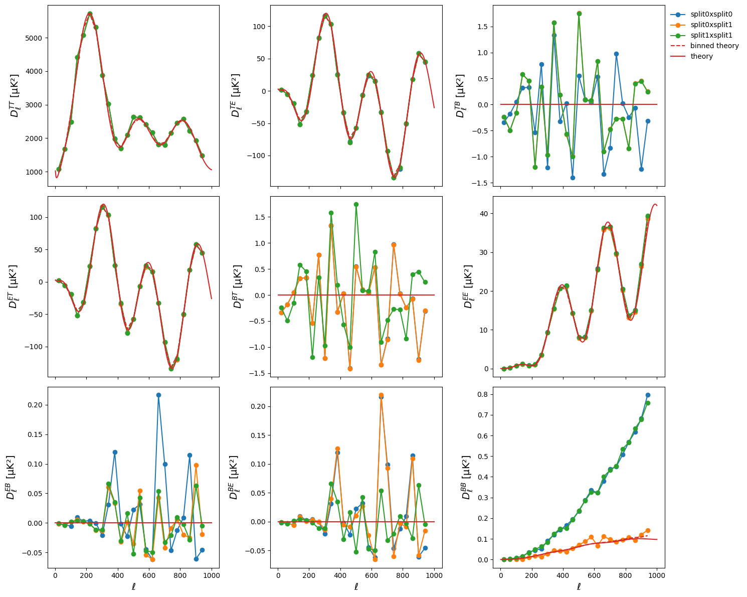
and we finally plot all the results

fig, axes = plt.subplots(3, 3, figsize=(15, 12), sharex=True)
for ax, spec in zip(axes.flatten(), spectra):
    for k, v in Db_dict.items():
        ax.plot(lb, v[spec], "-o", label=k)
    ax.plot(lb, ps_theory_b[spec], "--", color="tab:red", label="binned theory")
    ax.plot(l, ps_theory[spec], color="tab:red", label="theory")
    ax.set_ylabel(r"$D^{%s}_{\ell}$ [µK²]" % spec, fontsize=14)

for ax in axes[-1]:
    ax.set_xlabel(r"$\ell$", fontsize=14)
axes[0, -1].legend(loc="upper left", bbox_to_anchor=(1, 1))
fig.tight_layout()