Compute spectra for standard and pure B modes

Introduction

This tutorial illustrates the spectra computation for standard and pure B modes. We will only use the HEALPIX pixellisation to pass through the different steps of generation.

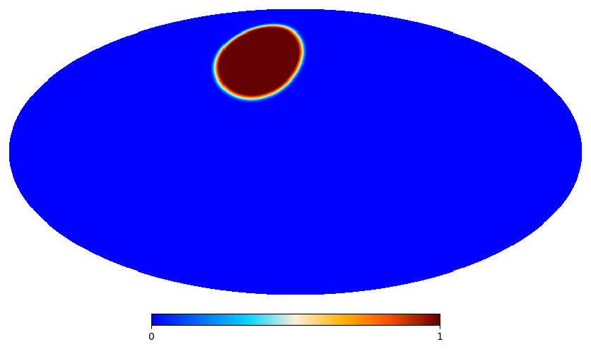
The HEALPIX survey mask is a disk centered on longitude 30° and latitude 50° with a radius of 25 radians. The nside value is set to 512 for this tutorial to reduce computation time.

Preamble

Versions used for this tutorial

import healpy as hp
import matplotlib as mpl
import matplotlib.pyplot as plt
import numpy as np
import pixell
import pspy

print("     Numpy :", np.__version__)
print("    Healpy :", hp.__version__)
print("Matplotlib :", mpl.__version__)
print("    pixell :", pixell.__version__)
print("      pspy :", pspy.__version__)

     Numpy : 1.26.3
    Healpy : 1.16.6
Matplotlib : 3.8.2
    pixell : 0.21.1
      pspy : 1.7.0+1.gafa4ce9.dirty

Set Planck colormap as default

pixell.colorize.mpl_setdefault("planck")

Generation of the templates, mask and apodisation type

We start by specifying the HEALPIX survey parameters namely longitude, latitude and patch size. The nside value is set to 512.

lon, lat = 30, 50
radius = 25
nside = 512

Given the nside value, we can set the \(\ell\)_max value

ℓmax = 3 * nside - 1

For this example, we will make use of 3 components : Temperature (spin 0) and polarisation Q and U (spin 2)

ncomp = 3

Given the parameters, we can generate the HEALPIX template as follow

from pspy import so_map

template = so_map.healpix_template(ncomp, nside)

We also define the binary template for the window function pixels

binary = so_map.healpix_template(ncomp=1, nside=nside)
vec = hp.pixelfunc.ang2vec(lon, lat, lonlat=True)
disc = hp.query_disc(nside, vec, radius=radius * np.pi / 180)
binary.data[disc] = 1

Generation of spectra

Generate window

We then create an apodisation for the survey mask. We use a C1 apodisation with an apodisation size of 5 degrees

from pspy import so_window

window = so_window.create_apodization(binary, apo_type="C1", apo_radius_degree=5)
hp.mollview(window.data, title=None)

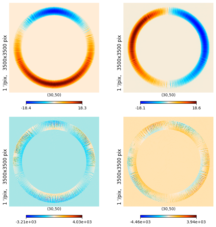
We can also have a look to the corresponding spin 1 and spin 2 window functions

niter = 3
w1_plus, w1_minus, w2_plus, w2_minus = so_window.get_spinned_windows(window, lmax=ℓmax, niter=niter)
plt.figure(figsize=(8, 8))
kwargs = {"rot": (lon, lat, 0), "xsize": 3500, "reso": 1, "title": None}
hp.gnomview(w1_plus.data, **kwargs, sub=(2, 2, 1))
hp.gnomview(w1_minus.data, **kwargs, sub=(2, 2, 2))
hp.gnomview(w2_plus.data, **kwargs, sub=(2, 2, 3))
hp.gnomview(w2_minus.data, **kwargs, sub=(2, 2, 4))

Binning file

We create a binning file with the following format : lmin, lmax, lmean

import os

from pspy import pspy_utils

output_dir = "/tmp/tutorial_purebb"
os.makedirs(output_dir, exist_ok=True)

binning_file = os.path.join(output_dir, "binning.dat")
pspy_utils.create_binning_file(bin_size=50, n_bins=300, file_name=binning_file)

Compute mode coupling matrix

For spin 0 and 2 the window need to be a tuple made of two objects: the window used for spin 0 and the one used for spin 2

window_tuple = (window, window)

The windows (for spin0 and spin2) are going to couple mode together, we compute a mode coupling matrix in order to undo this effect given the binning file. We do it for both calculations i.e. standard and pure B mode

from pspy import so_mcm

kwargs = dict(win1=window_tuple, binning_file=binning_file, lmax=ℓmax, niter=niter, type="Cl")

print("Computing standard mode coupling matrix")
mbb_inv, Bbl = so_mcm.mcm_and_bbl_spin0and2(**kwargs)

print("Computing pure mode coupling matrix")
mbb_inv_pure, Bbl_pure = so_mcm.mcm_and_bbl_spin0and2(**kwargs, pure=True)

Show code cell output Hide code cell output

Computing standard mode coupling matrix
Computing pure mode coupling matrix

Generation of ΛCDM power spectra

We first have to compute \(C_\ell\) data using a cosmology code such as CAMB and we need to install it since this is not a prerequisite of pspy. We can do it within this notebook by executing the following command

%pip install camb

Requirement already satisfied: camb in /home/garrido/Workdir/cmb/development/pspy/pyenv/lib/python3.11/site-packages (1.5.3)
Requirement already satisfied: scipy>=1.0 in /home/garrido/Workdir/cmb/development/pspy/pyenv/lib/python3.11/site-packages (from camb) (1.11.4)
Requirement already satisfied: sympy>=1.0 in /home/garrido/Workdir/cmb/development/pspy/pyenv/lib/python3.11/site-packages (from camb) (1.12)
Requirement already satisfied: packaging in /home/garrido/Workdir/cmb/development/pspy/pyenv/lib/python3.11/site-packages (from camb) (23.2)
Requirement already satisfied: numpy<1.28.0,>=1.21.6 in /home/garrido/Workdir/cmb/development/pspy/pyenv/lib/python3.11/site-packages (from scipy>=1.0->camb) (1.26.3)
Requirement already satisfied: mpmath>=0.19 in /home/garrido/Workdir/cmb/development/pspy/pyenv/lib/python3.11/site-packages (from sympy>=1.0->camb) (1.3.0)
Note: you may need to restart the kernel to use updated packages.

To make sure everything goes well, we can import CAMB and check its version

import camb

print("CAMB version:", camb.__version__)

CAMB version: 1.5.3

Now that CAMB is properly installed, we will produce the \(C_\ell\)s from \(\ell\)_min=2 to \(\ell\)_max=10⁴ for the following set of \(\Lambda\)CDM parameters

ℓ = np.arange(2, 10_000)
cosmo_params = {
    "H0": 67.5,
    "As": 1e-10 * np.exp(3.044),
    "ombh2": 0.02237,
    "omch2": 0.1200,
    "ns": 0.9649,
    "Alens": 1.0,
    "tau": 0.0544,
}
pars = camb.set_params(**cosmo_params)
pars.set_for_lmax(ℓ[-1], lens_potential_accuracy=1)
results = camb.get_results(pars)
powers = results.get_cmb_power_spectra(pars, CMB_unit="muK")

We finally have to write \(C_\ell\) into a file to feed the so_map.synfast function

cl_file = os.path.join(output_dir, "cl_camb.dat")
np.savetxt(cl_file, np.hstack([ℓ[:, np.newaxis], powers["total"][ℓ]]))

Running simulations

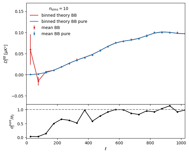
Given the parameters and data above, we will now simulate n_sims simulations to check for mean and variance of BB spectrum. For illustrative purpose, we will only run 10 simulations (~ few minutes) but for reasonable comparisons, you should increase this number to few tens of simulations.

We will do it for both calculations (standard and pure) and finally we will graphically compare results

We first need to specify the order of the spectra to be used by pspy although only BB spectrum will be used

spectra = ["TT", "TE", "TB", "ET", "BT", "EE", "EB", "BE", "BB"]

and we define a dictionnary of methods regarding the calculation type for B mode spectrum

from pspy import sph_tools

methods = {
    "standard": dict(alm=sph_tools.get_alms, mbb=mbb_inv),
    "pure": dict(alm=sph_tools.get_pure_alms, mbb=mbb_inv_pure),
}

from pspy import so_spectra
from tqdm.auto import tqdm

for _ in tqdm(range(n_sims := 10)):
    cmb = template.synfast(cl_file)
    for k, v in methods.items():
        get_alm = v.get("alm")
        alm = get_alm(cmb, window_tuple, niter, ℓmax)
        ℓ, ps = so_spectra.get_spectra(alm, spectra=spectra)
        ℓb, ps_dict = so_spectra.bin_spectra(
            ℓ, ps, binning_file, ℓmax, type="Cl", mbb_inv=v.get("mbb"), spectra=spectra
        )
        v.setdefault("bb", []).append(ps_dict["BB"])

Let’s plot the mean results against the theory value for BB spectrum

for k, v in methods.items():
    v["mean"] = np.mean(v.get("bb"), axis=0)
    v["std"] = np.std(v.get("bb"), axis=0)

ℓ_th, ps_theory = pspy_utils.ps_lensed_theory_to_dict(cl_file, output_type="Cl", lmax=ℓmax)
ps_theory_b = so_mcm.apply_Bbl(Bbl, ps_theory, spectra=spectra)
ps_theory_b_pure = so_mcm.apply_Bbl(Bbl_pure, ps_theory, spectra=spectra)

fac = ℓb * (ℓb + 1) / (2 * np.pi)
facth = ℓ_th * (ℓ_th + 1) / (2 * np.pi)

fig = plt.figure(figsize=(7, 6))
grid = plt.GridSpec(4, 1, hspace=0, wspace=0)

main = fig.add_subplot(grid[:3], xticklabels=[], xlim=(0, 2 * nside))
main.plot(ℓ_th[:ℓmax], ps_theory["BB"][:ℓmax] * facth[:ℓmax], color="grey")
main.errorbar(ℓb, ps_theory_b["BB"] * fac, color="tab:red", label="binned theory BB")
main.errorbar(ℓb, ps_theory_b_pure["BB"] * fac, color="tab:blue", label="binned theory BB pure")
main.errorbar(
    ℓb,
    methods.get("standard").get("mean") * fac,
    methods.get("standard").get("std") * fac,
    fmt=".",
    color="tab:red",
    label="mean BB",
)
main.errorbar(
    ℓb,
    methods.get("pure").get("mean") * fac,
    methods.get("pure").get("std") * fac,
    fmt=".",
    color="tab:blue",
    label="mean BB pure",
)
main.set(ylim=(-0.07, 0.17), ylabel=r"$D^{BB}_{\ell}$ [µK²]")
plt.legend(title=r"$n_{\rm sims}=%s$" % n_sims)

ratio = fig.add_subplot(grid[3], xlim=(0, 2 * nside))
ratio.plot(ℓb, methods.get("pure").get("std") / methods.get("standard").get("std"), ".-k")
ratio.set(ylabel=r"$\sigma^{\rm pure}_\ell/ \sigma_\ell$", xlabel=r"$\ell$")
ratio.axhline(1, color="gray", ls="dashed");