Read, write and plot maps#
Introduction#
This tutorial shows how to read/write and plot SO maps. We will use both pixellisation i.e. CAR and
HEALPIX with the same interface showing how pspy can deal with both data format.
Preamble#
Versions used for this tutorial
import matplotlib as mpl
import matplotlib.pyplot as plt
import numpy as np
import pixell
import pspy

print("     Numpy :", np.__version__)
print("Matplotlib :", mpl.__version__)
print("    pixell :", pixell.__version__)
print("      pspy :", pspy.__version__)
     Numpy : 1.26.3
Matplotlib : 3.8.2
    pixell : 0.21.1
      pspy : 1.7.0+5.g6447766
Set Planck colormap as default
pixell.colorize.mpl_setdefault("planck")
Generation of CAR and HEALPIX templates#
We start with the definition of the CAR template, it will go from right ascension ra0 to ra1 and
from declination dec0 to dec1 (all in degrees). The resolution will be 1 arcminute and we will allow
3 components (stokes parameter in the case of CMB anisotropies)
ra0, ra1, dec0, dec1 = -5, 5, -5, 5
res = 1
ncomp = 3
from pspy import so_map

template_car = so_map.car_template(ncomp, ra0, ra1, dec0, dec1, res)
We do the same with HEALPIX
template_healpix = so_map.healpix_template(ncomp, nside=256, coordinate="equ")
Simulation of CMB data#
We first have to compute the power spectra \(C_\ell\)s using a Boltzmann solver such as CAMB and we need to install it
since this is a prerequisite of pspy. We can do it within this notebook by executing the following
command
%pip install camb
Requirement already satisfied: camb in /home/garrido/Workdir/cmb/development/pspy/pyenv/lib/python3.11/site-packages (1.5.3)
Requirement already satisfied: scipy>=1.0 in /home/garrido/Workdir/cmb/development/pspy/pyenv/lib/python3.11/site-packages (from camb) (1.11.4)
Requirement already satisfied: sympy>=1.0 in /home/garrido/Workdir/cmb/development/pspy/pyenv/lib/python3.11/site-packages (from camb) (1.12)
Requirement already satisfied: packaging in /home/garrido/Workdir/cmb/development/pspy/pyenv/lib/python3.11/site-packages (from camb) (23.2)
Requirement already satisfied: numpy<1.28.0,>=1.21.6 in /home/garrido/Workdir/cmb/development/pspy/pyenv/lib/python3.11/site-packages (from scipy>=1.0->camb) (1.26.3)
Requirement already satisfied: mpmath>=0.19 in /home/garrido/Workdir/cmb/development/pspy/pyenv/lib/python3.11/site-packages (from sympy>=1.0->camb) (1.3.0)
Note: you may need to restart the kernel to use updated packages.
To make sure everything goes well, we can import CAMB and check its version
import camb

print("CAMB version:", camb.__version__)
CAMB version: 1.5.3
Now that CAMB is properly installed, we will produce \(C_\ell\) data from \(\ell\)min=2 to
\(\ell\)max=104 for the following set of \(\Lambda\)CDM parameters
ℓmin, ℓmax = 2, 10**4
cosmo_params = {
    "H0": 67.5,
    "As": 1e-10 * np.exp(3.044),
    "ombh2": 0.02237,
    "omch2": 0.1200,
    "ns": 0.9649,
    "Alens": 1.0,
    "tau": 0.0544,
}
pars = camb.set_params(**cosmo_params)
pars.set_for_lmax(ℓmax, lens_potential_accuracy=1)
results = camb.get_results(pars)
powers = results.get_cmb_power_spectra(pars, CMB_unit="muK")
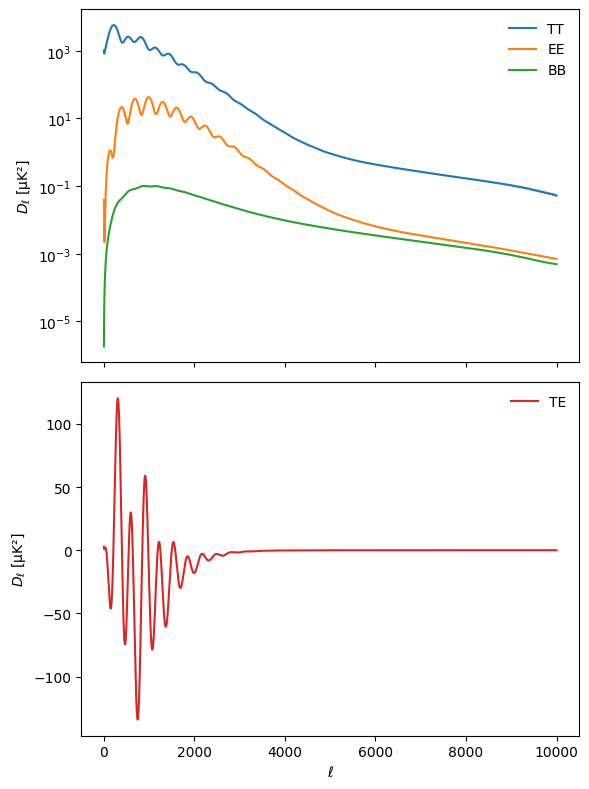
We can plot the results for sanity check
ℓ = np.arange(ℓmin, ℓmax)
cl_dict = {spec: powers["total"][ℓmin:ℓmax, i] for i, spec in enumerate(["tt", "ee", "bb", "te"])}
fig, axes = plt.subplots(2, 1, sharex=True, figsize=(6, 8))
axes[0].set_yscale("log")
for i, (k, v) in enumerate(cl_dict.items()):
    ax = axes[1] if k == "te" else axes[0]
    ax.plot(l, v, f"-C{i}", label=k.upper())

for ax in axes:
    ax.set_ylabel(r"$D_\ell$ [μK²]")
    ax.legend()
axes[1].set_xlabel("ℓ")
fig.tight_layout()
We finally have to write the \(C_\ell\)s into a file to feed the so_map.synfast function for both
pixellisation templates
import os

output_dir = "/tmp/tutorial_io"
get_output_path = lambda fname: os.path.join(output_dir, fname)


os.makedirs(output_dir, exist_ok=True)
cl_file = get_output_path("cl_camb.dat")
np.savetxt(cl_file, np.hstack([ℓ[:, np.newaxis], powers["total"][ℓmin:ℓmax]]))

cmb_car = template_car.synfast(cl_file)
cmb_healpix = template_healpix.synfast(cl_file)
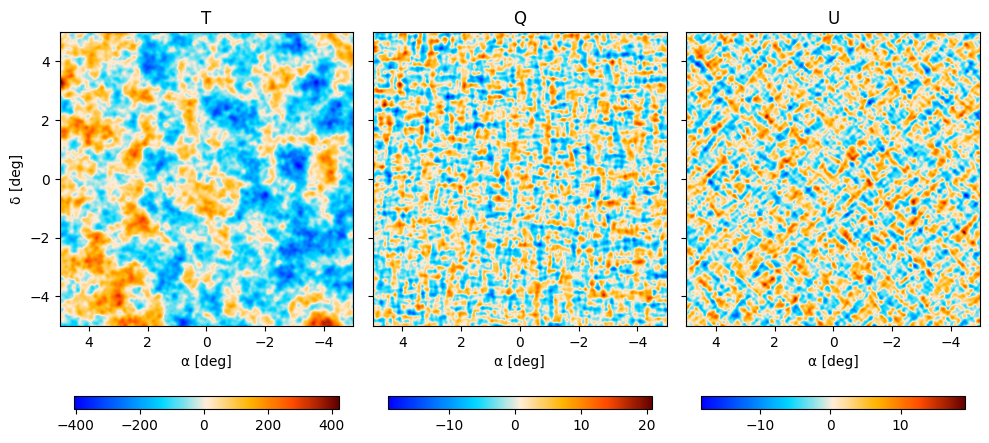
We can plot both maps, first for the CAR pixellisation
fig, axes = plt.subplots(1, 3, figsize=(10, 5), sharey=True)
kwargs = dict(extent=[ra1, ra0, dec0, dec1], origin="lower")
for i, field in enumerate(fields := "TQU"):
    im = axes[i].imshow(cmb_car.data[i], **kwargs)
    axes[i].set_title(field)
    fig.colorbar(im, ax=axes[i], orientation="horizontal", shrink=0.9)

axes[0].set_ylabel("δ [deg]")
for ax in axes:
    ax.set_xlabel("α [deg]")
fig.tight_layout()
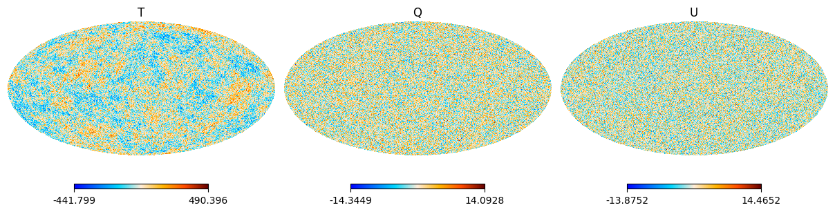
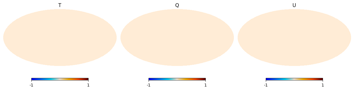
then for the HEALPIX pixellisation
import healpy as hp

plt.figure(figsize=(12, 8))
for i, field in enumerate(fields):
    hp.mollview(cmb_healpix.data[i], title=field, sub=(1, ncomp, i + 1))
Actually, saving CMB maps can be done with the so_map.plot function which can be used interactively
(maps will popup via an external image viewer program) but can also be used to store each CMB maps
(T, Q, U) inside a directory as follow
cmb_car.plot(file_name=get_output_path("map_car_io"))
cmb_healpix.plot(file_name=get_output_path("map_healpix_io"))
Writing/reading SO maps#
Maps can also be writen to disk in fits format with the so_map.write_map function
cmb_car.write_map(get_output_path("map_car.fits"))
cmb_healpix.write_map(get_output_path("map_healpix.fits"))
Show code cell output
setting the output map dtype to [dtype('float64'), dtype('float64'), dtype('float64')]
We can read them back
cmb_car2 = so_map.read_map(get_output_path("map_car.fits"))
cmb_healpix2 = so_map.read_map(get_output_path("map_healpix.fits"))
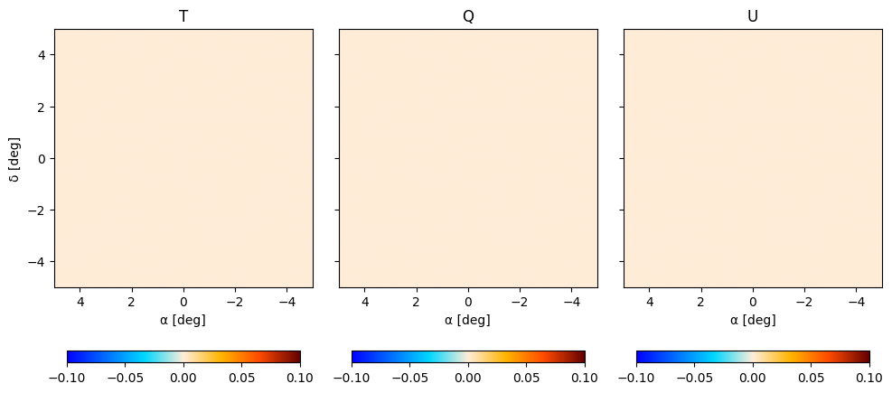
We null them
cmb_car2.data -= cmb_car.data
cmb_healpix2.data -= cmb_healpix.data
and plot the nulls
fig, axes = plt.subplots(1, 3, figsize=(10, 5), sharey=True)
for i, field in enumerate(fields):
    im = axes[i].imshow(cmb_car2.data[i], **kwargs)
    axes[i].set_title(field)
    fig.colorbar(im, ax=axes[i], orientation="horizontal", shrink=0.9)

axes[0].set_ylabel("δ [deg]")
for ax in axes:
    ax.set_xlabel("α [deg]")
fig.tight_layout()
plt.figure(figsize=(12, 8))
for i, field in enumerate(fields):
    hp.mollview(cmb_healpix2.data[i], title=field, sub=(1, ncomp, i + 1))
np.allclose(cmb_car2.data, 0), np.allclose(cmb_healpix2.data, 0)
(True, True)